Documentation of the Bifrost model estimation of parameters used for modifying CapTool to account for recent changes in the Barents Sea
Sigurd Tjelmeland
Printed {2013, 12, 10, 9, 38, 30.8424775}
This document is an expanded version of the Working document WD1 to the capelin subgroup of the Arctic Fisheries WG that took place in Svanhovd, October 1-2 2012. Many figures showing diagnostics of the model used at Svanhovd have been removed for clarity and the model has been expanded to include consumption by cod also in quarters 2 and 3, and to include cod cannibalism. Results of the new model are presented and compared to the Svanhovd 2012 version.
In addition, recruitment relations are estimated and used in long term simulations that can be used for estimating optimal harvest rules in the cod-capelin-herring system of the Barents Sea.
The document contains material that can be used in a new Stock Annex for the Barents Sea capelin, but in addition also describes more technical handling of the software.
Introduction
The Barents Sea capelin is surveyed once a year in September, in a joint Russian-Norwegian trawl-acoustic survey. The data from this survey in the form of number of capelin at age and length and weight at length are the most important scientific basis for the management.
As for most fish stocks, the management goal is to keep the spawning stock biomass high enough for the recruitment not to be unduly hampered, which is implemented by quotas that secure a minimum probability of 0.95 for the spawning stock biomass to be larger than 200 000 tonnes. These reference values are set by ICES (by the formerly ACFM).
The latest years ICES has undertaken work to supplement the Precautionary Approach with MSY-based management, i.e. building harvest rules that seek to maximise a long-term goal instead of avoiding recruitment failure next year. The Joint Russian-Norwegian Fisheries Commission has decided to evaluate the harvest rules for Barents Sea species in 2015 and a possible change of the present harvest rule will be deferred until then.
The present document describes modifications to the management models needed in order to cope with the changing ecological situation in the Barents Sea that to a large extent makes some of the assumptions underlying the present (used in 2011) model invalid. This is commented on the ICES advice sheet in the autumn 2011.
This document is written for an audience that is familiar with the management of Barents Sea capelin and the modelling underlying it.
It should be noted that the assessment of capelin includes estimating parameters in models for the population dynamics, unlike many other stocks where the population dynamics is represented by the constant parameter M, which usually is not estimated. The basic problems are:
Determining the functional form for maturation
Determining the functional form for consumption
Selecting distribution functions for data used in the likelihood function
For long term simulations needed to test harvest rules the basic problem is to select proper recruitment relations, where the recruitment is determined by the spawning stock biomass and appropriate other covariates. This document shows how this can be done by devising a large number of plausible recruitment relations and selecting those to be used in prognostic simulation from statistical criteria. In addition, it is shown how models for weight at age and maturity at age can be estimated from historic data and used in long term simulations. In all these models there are environmental drivers, so that one can test consequences of hypotheses about future change of the environment.
The problem
The scientific challenge is two-fold, or rather two-staged. Firstly, a model must be established from which one can make probabilistic projections of spawning biomass at the spawning time from the measurment of the total stock by age and length by October 1. Secondly, relations between the historic spawning biomass and recruitment must be established, to drive the testing of harvest rules by long term simulation.
Testing of the present and other harvest rules are deferred to 2015, when the Barents Sea harvest rules will be looked upon anew from the management side.
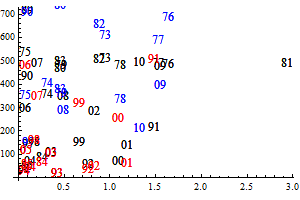
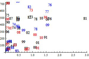
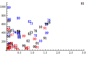
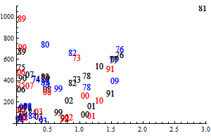
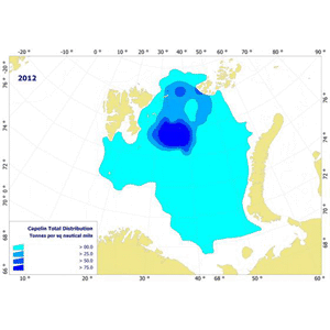
In recent years there have been a record northerly distribution of the cod at the September survey, with full overlap of large parts of the capelin distribution (figure )1. This results in high predation during late autumn and long routes of co-migration for both species towards the spawning grounds. Traditionally, the management of capelin has relied on the assumption that the consumption by cod of immature capelin during January-March is very small compared to the consumption of mature capelin, and that the consumption of capelin by mature cod (migrating towards the spawning grounds) is very small compared to the consumption by immature cod. At the assessment meeting in 2011 the possible inadquacy of these assumptions was pointed out, as was the inadequacy of the habit of basing the natural mortality during October-december on estimated natural mortality of capelin, distributed evenly throughout the year. At the assessment meeting in 2012 an alternative assessment using a model where these assumptions were lifted. This assessment would have given a lower quota advice (140 000 tonnes as opposed to 200 000 tonnes). The present document describes a further elaborated version of the 2012 model.
 |
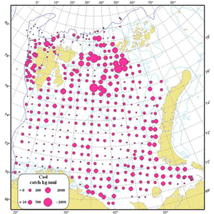 |
Figure 1. Geographical distribution of capelin (left) and cod (right) in the autumn 2012.
Model rigging
The estimation of parameters for capelin maturation and consumption of capelin by cod is done in the model Bifrost, which is written in Mathematica. In order to have a simpler tool for the yearly quota calculations the parameters are copied to the Excel-based field model CapTool, which uses the add-on module @RISK for stochastic simulations.
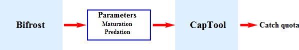
Figure 1. Relation between the models Bifrost and CapTool
The data
There is a wide variety of data behind the estimation of parameters in the population model, and to a large extent raw data are used. The data are processed with separate programs before read into Bifrost.
Survey data of capelin in September
Since 1972 the Barents Sea has been surveyed for capelin in September, from 1978 as a joint Russian-Norwegian effort. The result is an abundance estimate in numbers by age by length on the spreadsheet CapTab, which is read by Bifrost at initialization time.
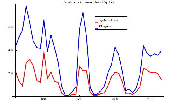
Figure 2. Historic biomass estimates of Barents Sea capelin
Consumption per cod
The parameters are estimated by building a likelihood function where the consumption per cod from the simulation are treated as expectation values and exogeneously calculated consumption per cod as data in a distribution function. Different functional forms are tested. The exogeneously calculated consumption per cod uses the following data:
-Stomach content data
-Evacuation rate data
-Temperature data
-Cod distribution data for a posssible weighting by area.
The consumption per cod is pre-calculated using an evacuation rate model without initial stomach content, and several replicates are made to account for uncertainty.
Stomach content data
Methods for geographical weighting
It is not apriori given that the stomach content data are sampled in proportion to the geographically structured abundance of cod in the sea. There are four different methods to deal with a possibly skewed sampling:
-Doing nothing
-Weight stomach content data according to the number of cod in each trawl station, as taken from the stomach content data base
-Weight each cod stomach with the number of cod in the same length group from the survey, meaned over geographical surroundings
-Base the weighting on survey estimate over Multspec areas
The survey estimates are made with Bifrost-related software using swept area. Figure 3 and figure 4 give an overview of the consumption per cod data available for the model.
Model selection
For very many processes there may be alternative model choices. Also, it is tempting to introduce extra parameters in order to get better fit to the data. In this document alternative models are compared using the small-sample Aikaike Information Criterion (AIC, Burnham and Anderson 1998, p66) to ensure parsimonous model selection.
The model
The model is called Bifrost (Boreal Integrated Fish Resource Optimisation and Simulation Tool), which also is the Norse name for the rainbow, believed to bridge two different worlds (see Snorre Sturlason's Edda from about 1220). Bifrost has evolved from the mid-1980s (then called CAPELIN, later evolved into a geographically distributed model called Multspec) and has been used in practical management for two decades, delivering parameter values to the Excel based field tool CapTool. The model has traditionally comprised consumption of mature capelin by immature cod in the pre-spawning period January-March.
Changing ecology - new challenges. The view of the autumn 2011
Changing ecological conditions led to extreme northwards distribution in the autumn for both cod and capelin with correspondingly long migration routes to the spawning areas for both stocks. It has therefore become evident that the two basic assumptions of mature cod not consuming capelin during January-March and cod consuming only mature capelin during January-March could not hold. Moreover, the large increase of the cod stock - particularly the mature part of the stock - makes a violation of these assumptions more severe.
Yet another fundamental assumption is that the natural mortality of mature capelin during October-December is equal to the natural mortality of immature capelin during the same period (although differemig from year to year). This assumption may still hold, but in order to evaluate the natural mortality of mature capelin during October-December it has been assumed that the observed yearly natural mortality of immature capelin coudl be divided evenly on each month. A large overlap between capelin and cod in the autumn in recent years combined with the fact that there has been no substantial increase in the estimated yearly natural mortality of immature capelin, leads to the conclusion that the assumption of a natural mortality evenly distributed throughout the year may not hold.
A revision of the model used for managing the capelin stock is thus called for, where the consumption of capelin by cod during October-December and the consumption of capelin by mature cod and the consumption of immature capelin during January-March are accounted for.
A preliminary version of a revised model was run experimentally at the assessment meeting in 2012 but was not adopted due to lack of ICES benchmarking.
The predation parameters for quarter 4 are also applied for quarter 2, quarter 3 and January. Predation parameters for quarter 4 being applied to January accounts for some of the consumption of capelin by mature cod in quarter 1 and for some of the consumption of immature capelin in quarter 1.
Overview of parameters
| Parameter software name | Parameter number | Parameter group | Time period in estimation |
| capelinP1Females | Maturation parameter | Early part | |
| capelinP2Females | Maturation parameter | Early part | |
| maxConsCodQ1 | Consumption parameter | Whole period | |
| maxConsCodQ4 | Consumption parameter | Whole period | |
| halfConsBiomassQ1 | Consumption parameter | Whole period | |
| halfConsBiomassQ4 | Consumption parameter | Whole period | |
| otherFoodCodQ1 | Consumption parameter | Whole period | |
| otherFoodCodQ4 | Consumption parameter | Whole period | |
| speciesSuitabilityCapelinCodQ1 | Consumption parameter | Whole period | |
| speciesSuitabilityCapelinCodQ4 | Consumption parameter | Whole period | |
| speciesSuitabilityCodCodQ1 | Consumption parameter | Whole period | |
| speciesSuitabilityCodCodQ4 | Consumption parameter | Whole period | |
| partImmaturePreyedByCodWinter | Consumption parameter | Whole period | |
| partMatureCodPreyingOnCapelinWinter | Consumption parameter | Whole period | |
| codWeightExponent | Consumption parameter | Whole period | |
| capelinAge1Addition | Yearly parameter | 1 year | |
| capelinMCorrection | Yearly parameter | 1 year | |
| codRecruitmentCorrection | Yearly parameter | 3 years |
First modelling step: mature capelin by October 1
The degree of maturation is determined by the length.
![]()
![]()
![]()
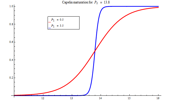
Figure 3. Bifrost maturation model.
A note on biology
The spawning predominantly occurs around 1 April, and sometimes earlier. However, a part of the stock may spawn in June. This stock component is largely unknown but may have an impact on recruitment. Furthermore, a summer-spawning component will largely be protected from the January-March fishery. This is not modelled in Bifrost yet ecause of lack of data for estimation but may be an effect that might have some impact on management and could be pursued in the future.
Second modelling step: consumption of capelin by cod
There are two alternative functional forms for consumption by cod, either:
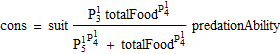
or:
![]()
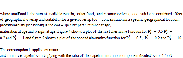
Figure 4. Bifrost consumption model.

Figure 5. Bifrost consumption model with free inflection point.
The cod dependent part: predationAbility
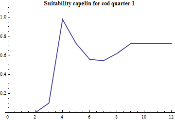
The capacity for consumption depends on cod age, but is not assumed a linear function of individual weight. The part of the consumption by cod that depends on the structure of the cod stock is given for capelin in quarter 1 as:
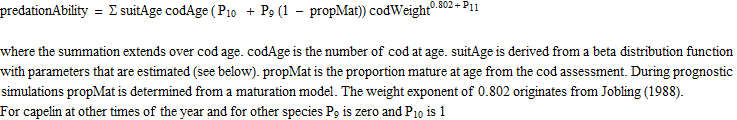
Suitability
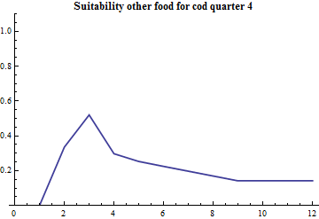
The term "suitability" is used for modfifications of the mathematical form(s) above to account for variation in geographical overlap between species, possible age-dependent variations in time and space of vertical migration that affect the predation and size effects. For each species there is a parameter that determines the overall suitability relative to other food and a vector over cod age that determines the size selectivity.
Species-specific suitability: suit
The species-specific suitability for other food is set to one, and the species-specific suitability for capelin and cod are estimated. For capelin the suitability modification from capelin and cod being partly separated in quarter 1 is handled explicity by splitting out the amount of cod assumed to be in the Svalbard area during this period.
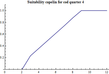
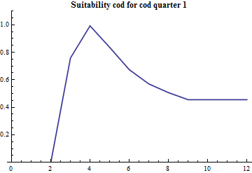
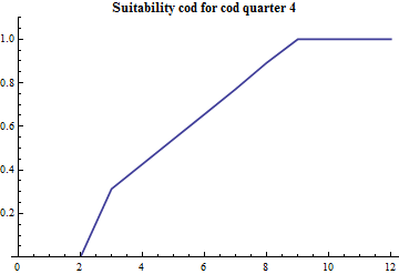
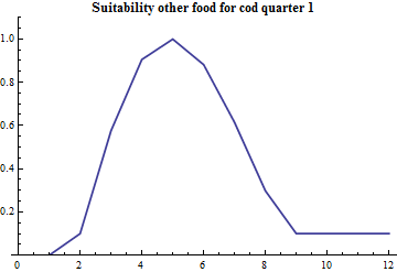
Age-specific suitability: suitAge
Since the part of mature cod that preys on capelin during the first quarter is estimated along with the other consumption parameters the age specific suitability is crucial since the abundance by age distinguished mature and immature capelin. The age specific suitability is modelled with 4 parameters: the suitability at lower and upper ages and the two parameters in the PDF of a beta distribution. The beta distribution does not have a statistical meaning in this case, it is just conveniently borrowed since it is bounded at both ends and there is built-in software for it's calculation and plotting. The realized suitabilities dependent on cod age are:
 |
 |
 |
 |
 |
 |
The modification of the model in quarter 1:
The overlap between capelin and cod, and the consumption for a given overlap, is in quarter 1 to a large degree determined by the biology connected to the spawning migration of both cod and capelin. In the context of management of capelin the model comprises only one crude adaption to spawning migration specific overlap variation: a part of the total cod stock is supposed to reside in the Svalbard area in quarter 1, not preying on capelin. In the present situation with a large ice free area in quarter 1, this assumption might be looked upon with fresh eyes. The Svalbard component is assessed by comparing the geographical distribution of cod in the autumn and the winter.
The model as used before 2012 was based on two assumptions that in recent years have been severely challenged: The consumption of capelin in quarter 4 is by mature cod only, and the cod eats only mature capelin in quarter 4. These assumptions may not be valid, especially in the present ecological situation with as extreme northwards distribution of both species in the autumn with as subsequent long route of co-migration.
The cod preys on capelin, cod and other food. The amount of other food is assumed constant.
A constant portion of mature cod preying on capelin in quarter 1 can is estimated as a parameter in the model, although it would be preferable to have exogeneous information.
The part of immature capelin that is consumed by cod in quarter 1 is also made a parameter to be estimated, although also here exogeneous information would be preferable.
As a default, the suitability of capelin as food for mature capelin is set to 0.5, but deviation from this assumption is tested.
Parameter connectivity
The parameters other than yearly parameters and the parameters governing growth and recruitment during prognostic simulations are shown in the table below, with their software names, which are self-explanatory, and their numbering as used in figures. These are the parameters that determine the perception of the historic spawning biomass. Estimating these parameters constitute the main part of the assessment of the stock.
| Parameter software name | Parameter number | Parameter group | Time period in estimation |
| capelinP1Females | Maturation parameter | Early part | |
| capelinP2Females | Maturation parameter | Early part | |
| maxConsCodQ1 | Consumption parameter | Whole period | |
| maxConsCodQ4 | Consumption parameter | Whole period | |
| halfConsBiomassQ1 | Consumption parameter | Whole period | |
| halfConsBiomassQ4 | Consumption parameter | Whole period | |
| otherFoodCodQ1 | Consumption parameter | Whole period | |
| otherFoodCodQ4 | Consumption parameter | Whole period | |
| speciesSuitabilityCapelinCodQ1 | Consumption parameter | Whole period | |
| speciesSuitabilityCapelinCodQ4 | Consumption parameter | Whole period | |
| speciesSuitabilityCodCodQ1 | Consumption parameter | Whole period | |
| speciesSuitabilityCodCodQ4 | Consumption parameter | Whole period | |
| partImmaturePreyedByCodWinter | Consumption parameter | Whole period | |
| partMatureCodPreyingOnCapelinWinter | Consumption parameter | Whole period | |
| codWeightExponent | Consumption parameter | Whole period | |
| capelinAge1Addition | Yearly parameter | 1 year | |
| capelinMCorrection | Yearly parameter | 1 year | |
| codRecruitmentCorrection | Yearly parameter | 3 years |
Figure 6 shows the parameter connectivity and how the value of each parameter influences the spawning stock biomass. If an increase of one parameter would lead to a change in the likelihood that could be counteracted by a decrease of another parameter, the connection line is blue. If it could be counteracted by an increase of the other parameter, the connection line is red. If the spawning stock biomass increases with the value of a parameter, the connection line to the spawning stock biomass is red, if it decreases, the connection line is blue.
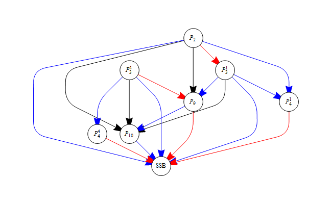
Figure 6. Parameter connectivity in Bifrost.
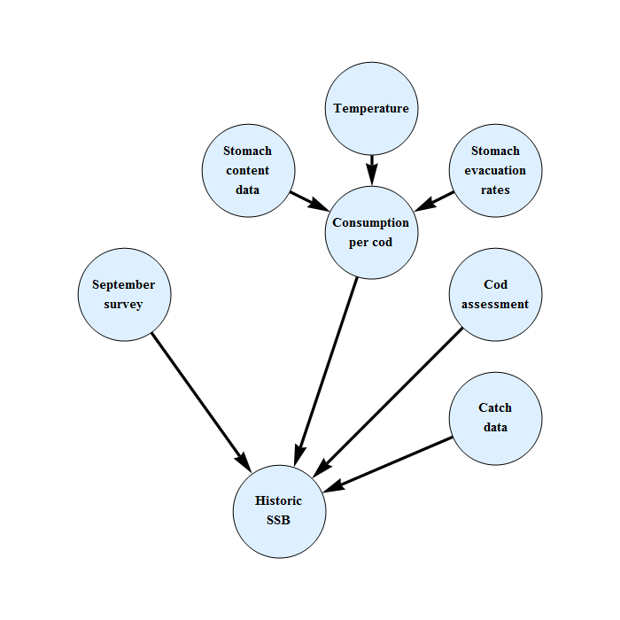
Estimation of parameters for the historic assessment
Even if care is taken to simplify the model as much as possible, the estimation task is difficult because there are several confounding parameters. Also, the CPU time used is an issue since a simulation throughout a significant part of the historic range usually is needed for each iteration of the estimation loop. A practical estimation scheme has proven to be to divide the estimation task into three parts. The maturation parameters are estimated using only the first part of the historic time series, from 1972 until a selectable year around 1980. In this period it is assumed that the predation of immature capelin by cod is a part of the residual natural mortality, which is assumed constant throughout the historic period used for estimation and which is estimated along with the maturation parameters. The next step is an estimation of predation mortalities using the historic time series from 1984, the first year of stomach content data. The estimation of predation parameters is based on a likelihood constructed from consumption per cod by cod age, where the data part is emprical calculation based on stomach content samples and laboratoty measured evacuation rates. The final step is to estimate yearly parameters for residal natural mortality for immature capelin, recruitment of cod as 0 year old and recruitment of capelin as 1 year old. The latter is measured but in the early parts of the time series have proved to be unreliable. This 3-step estimation is carried out iteratively until convergence since there is some feedback from the two latter steps to the first step.
Likelihood
Parameter estimation is based on maximum likelihood throughout, and the uncertainty parameters in the selected distributional functions are estimated along with the other parameters. This enables use of Akaike's information criterion to select the most parsimonous model from a suite of candidate formulations of the basic biological processes.
Compatibility of data
The main problem in the estimation of parameters is to find a set of parameters that lead to non-vanishing SSBs and positive residual mortalities.If such a set does not exist, there must be some incompatibility between the main data sources.
Custom estimation method
When the predation in quarter 4 is estimated the built-in estimation programs in Mathematica do not work properly, for some reason or other. Therefore a custom method is implemented, in which the minimum for one parameter at a time is found, diminishing the search area progressively.
Also, estimation of predation in quarter 4 confounds the parameters governing predation and parameters governing maturation of capelin. For this reason, and for the reason of having a model as compatible as possible with previous models, it is assumed that predation of capelin in quarter 1 of capelin by mature cod, starts gradually in 1984 and has its full strength in 1994. The same assumption is made for cod preying immature capelin in quarter 1.
In order to secure a swift and gracious convergence to the likelihood maximum, the order of parameter variation has been chosen so that the parameters (e.g. other food) pertaining to quarter of year are varied before global parameters (e.g. maximum consumption rate).
The estimation is performed with three operations in sequence, estimation of maturation parameters for capelin, estimation of predation parameters and estimation of yearly (residual M, number of age 1 capelin, number of age 0 cod) parameters. This sequence is performed iteratively until convergence.
The model is run only for the period of interest for the specific parameter group. Figure 7 shows a sketch of the procedure.
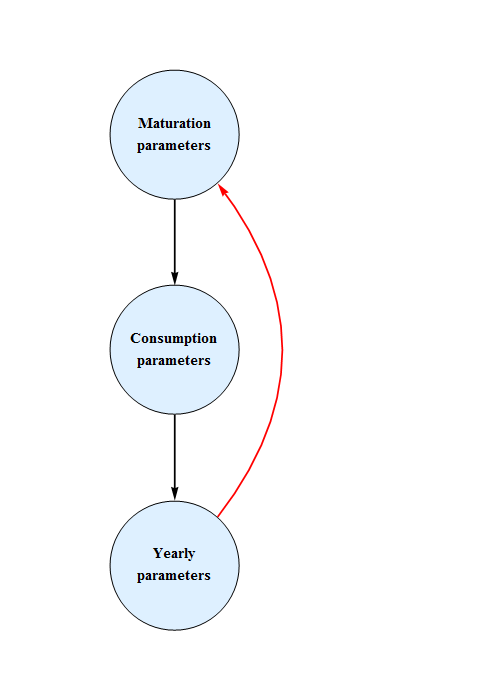
Figure 7. Estimation sequence in Bifrost.
It should be verified that the esimation sequence in fact converges.
During the estimation of the consumption parameters the likelihood terms when the maturation parameters and recruitments are estimated are ommitted, since in the present rigging of the estimation procedure the appropriate time period is not included (to save time) and justifies since the consumption parameters do not influence the maturation parameters. During the estimation of the yearly parameters neither the likelihood terms for the maturation parameters nor the likelihood terms for the predation parameters are invoked. It is only the value of the objective function for the consumption parameters and the residual M for capelin that is stored and reported across iterations.
Biological assumptions
In way of simplification of the estimation, several assumptions concerning the biology of the ecosystem have been made. These are explained in later chapters. An overview is given in the table below.
| Assumption | Comment |
| The maturation parameters do not change over time | Only the period 1973-1981 have been used in estimation of maturation parameters. This is a period of more stability of M on immature capelin, the estimation of which is confounded with the estimation of maturation parameters. |
| Maturation by length does not change by age | This is not true judged from empirical maturation data from the autumn. However, it is a reasonable simplifying assumption to keep the number of parameters to be estimated down. Bifrost provides for a lifting of this constraint at the next update. |
| Males and females have the same population biolog | This is not true, as both maturation and growth differ by sex. However, this approximation which Bifrost provides for may be lifted at the next update, is made in order to keep the number of parameters to be estimated down. |
| Residual natural mortality does not depend on age or sex | To the extent non-cod predators discriminates beween sex or age this is not true. This may happen if there are systematic differences in geographical overlap. |
Choice of error distribution
When parameters are estimated by maximising a likelihood function, a distribution for the data must be specified. The distribution most commonly used is the log-normal distribution. This is also the distribution used de facto when a likelihood is not used, but logarithms are taken before the estimation is carried out, which is far too frequently the case in fisheries research. In this document both the log-normal distribution and the gamma distribution have been tested, with radically different results. Figure 7 shows a plot of these distributions.
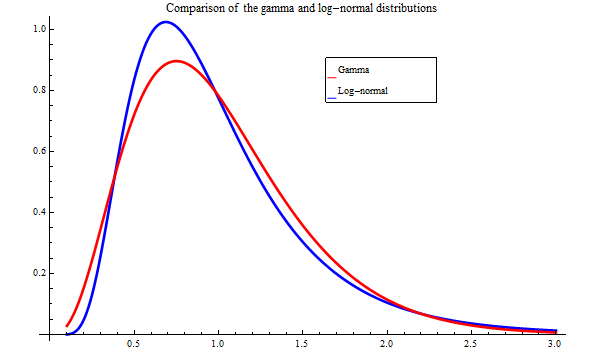
Figure 7. The gamma and log-normal distributions for an expectation value of 0.1. The CV of the gamma distribution is 0.5. The standard deviation of the log-normal distribution is 0.5, which also is close to the CV
The gamma distribution is "fatter" than the log-normal distribution, and is more tolerable to measurements deviation from the centre of the distribution.
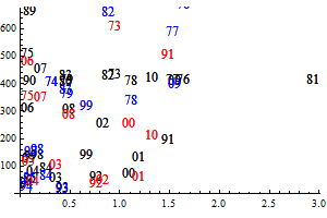
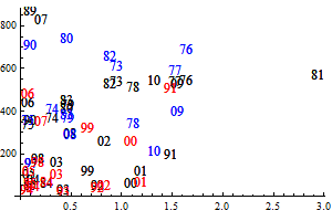
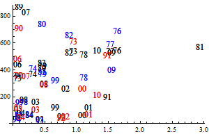
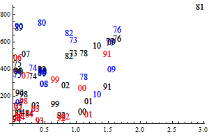
Consumption data
The stomach data used for quarter 1 are largely taken from the demersal survey in this period. It is possible that a substantial part of the consumption happens in January when there are fewer stomach samples than in February and March.
 |
 |
 |
Figure 8. Consumption per cod by station in 2010, Quarter 1 (left), quarter3 (middle) and quarter 4 (right)
The distribution in quarter 4 resembles the distribution in quarter 1. However, the north-east part of the Barents Sea is to a large extent outside of the surveyed area. Thus, it could be a possibility to combine stomach samples from quarter 3 and quarter 4 for use in quarter 4 because the large northwards distribution towards the end of quarter 3 means that both cod and capelin must be present in the northeast part of the sea at least in parts of quarter 4. However, for simplicity the stomach samples used are solely those from quarter 4.
The likelihood function
Empirical consumption of capelin by cod
Consumption of immature cod in quarter 1
Although the emprical consumption of capelin per cod calculations are made conditionally on capelin length, experience shows that it may be difficult to use this to distinguish between consumption on mature and immature capelin in the data entering the likelihood function. This is because the emprical data in the likelihood function become functions of model parameters. Also, there are few capelin in the cod stomachs being length measured, further increasing the problems. Therefore, the distinction beteen consumption on immature and mature capelin will be made in the simulation only, and the empirical data in the likelihodd will be for all capelin consumed.
Penalizing?
The consumption parameters may be strongly confounded with the maturation parameters if all parameters are estimated simultaneously. Increasing length at maturity leads to decreased mature stock, thereby increasing the consumption parameters for the modelled consumption to match the empirical consumption, decreasing SSB further. The end result may be a marginal improvement in likelihood, but a large decrease of SSB. Earlier versions of Bifrost avoided this problem by estimating length at maturity in a first step, independently of the predation parameters. If we want to estimate all parameters simultaneously, we might solve this problem by invoking a penalty that secure non-vanishing SSB.
However, for simplicity and for being as compatible with the earliet version underlying present management, the maturation parameters will be estimated in a separate step, although built-in in an iterative estimation of the parameters, see further explanations below.
Scaling capelin?
It is a well-known problem that combining the capelin acoustic estimate with consumption by cod based on stomach samples may lead to vanishing spawning stocks of capelin - understocking. This may happen in Bifrost in the beginning of the 1970s when the predation model is based on the stomach samples collected from 1984. The problem may lie in time dependency of the parameters governing the maturation, but the possibility that the acoustic estimate of capelin is an underestimate can not be ruled out.
Also, in several years cohorts that are simulated from 1 October one year (as immature fish determined from the survey estimate and the maturation model) to October 1 next year may be smaller than the survey estimate of the cohort. In those cases the predation in quarter 4 of the immature capelin is so large that there is no room for a residual mortality that can account for predation of capelin by mammals.
As is the case for most other stocks, it might be possible to treat the capelin survey as an index. However, then the use of the biomass reference point should be re-thought. In a later chapter there is a more comprehensive discussion of the understocking problem.
Compound error distribution?
The default approach to handling error distribution is to assume one form and estimate the uncertainty parameter along with the other parameters. However, there is not only uncertainty in the data used in the likelihood, there is also uncertainty in the expectation values because they originate in the September survey data. There is uncertainty in these data, which is a part of the likelihood. It would be logical then to confound an error distribution for e.g. consumption per cod with the current error applied for the September data, i.e. use a compound error distribution. This might be done in a future experiment but is not attempted here.
Estimation of the amount of mature cod preying capelin during January-March
Not all cod that might be considered mature on basis of length or age will every year migrate to the south-west to spawn. The ratio of the number of mature cod to the number of immature cod per length group as function of longitude is increasing in some years and decreasing in other years, but not much however.
Basing the estimation of how large part of the mature cod stock preying capelin during January-March on the stomach samples collected during this period proves difficult or may lead to wrong results because the stomach content samples are mostly collected inside the Barents Sea, where only a small part of the mature cod stock may reside at this time. An option is to calculated the amount of mature cod inside the Barents Sea that preys capelin in relation to the amount of immature capelin.
Penalty on vanishing SSB
In many estimation variants the capelin SSB becomes zero, i.e. the mature biomass at January 1 is not large enough to account for catch and consumption by cod during January-March. This does primarily happen during during the first part of the 1970s. There was recruitment in all years, so this does not correspond to any biological reality. Either the consumption model is wrong for this period or there is bias in one of the fundamental data sources used for estimating consumption: The capelin survey, the cod assessment or the stomach evacuation rates determined in the laboratory. The latter possibility is dealt with by applying a scaling factor to each of these data sources, and select the factor combination that is most likeliy according to the value of the likelihood function.
It is difficult to check the consumption model for the 1970s, as there are no stomach samples. There is a distinct possibility that the consumption by cod during January-March could be highly depensatory, wich is investigated in estimation experiments.
The capelin SSB deficiency is defined as the consumption on mature capelin that would have occured after the mature capelin biomass became 0, if the consumption continued with the average consumption per time step that occurred before the mature biomass became zero. This entity is used when the penalty is constructed.
Estimation variants
There are many different plausible assumptions that may be made. Selecting the final set may be based on the values of the likelihood and the number of parameters using the Akaike criterion, or by judging the reasonableness of other diagnostics. Another aspect to consider is the reasonableness of the estimation results, e.g. vanishing SSBs and negative residual M show that there is something wrong.
{Whether default, File likelihoodComponents, }
does not exist
{Whether default, File likelihoodComponents, , }
does not exist
{Whether default, File likelihoodComponents, , , }
does not exist
{Whether default, File likelihoodComponents, , , , Default}
does not exist
| Whether default | File likelihoodComponents does not exist |
Default | |||||||||||||||||||||||||||||||||||||||||||||||||||||||||||||||||||||||||||||||||||||||||||||||||||||||||||||||||||||||||||||||||||||||||||||||||||||||||||||||||||||||||||||||||||||||||||||||||||||||||||||||||||||||||||||||||||||||||||||||||||||||||||||||||||||||||||||||||||||||||||||||||||
| Fixed addition to P2 for age 2 | x | ||||||||||||||||||||||||||||||||||||||||||||||||||||||||||||||||||||||||||||||||||||||||||||||||||||||||||||||||||||||||||||||||||||||||||||||||||||||||||||||||||||||||||||||||||||||||||||||||||||||||||||||||||||||||||||||||||||||||||||||||||||||||||||||||||||||||||||||||||||||||||||||||||||
| Estimation of parametric cod-capelin suitability | x | x | x | x | x | ||||||||||||||||||||||||||||||||||||||||||||||||||||||||||||||||||||||||||||||||||||||||||||||||||||||||||||||||||||||||||||||||||||||||||||||||||||||||||||||||||||||||||||||||||||||||||||||||||||||||||||||||||||||||||||||||||||||||||||||||||||||||||||||||||||||||||||||||||||||||||||||||
| Estimation of parametric cod-cod suitability | x | x | x | x | x | ||||||||||||||||||||||||||||||||||||||||||||||||||||||||||||||||||||||||||||||||||||||||||||||||||||||||||||||||||||||||||||||||||||||||||||||||||||||||||||||||||||||||||||||||||||||||||||||||||||||||||||||||||||||||||||||||||||||||||||||||||||||||||||||||||||||||||||||||||||||||||||||||
| Estimation of parametric cod-other food suitability | x | x | x | x | x | ||||||||||||||||||||||||||||||||||||||||||||||||||||||||||||||||||||||||||||||||||||||||||||||||||||||||||||||||||||||||||||||||||||||||||||||||||||||||||||||||||||||||||||||||||||||||||||||||||||||||||||||||||||||||||||||||||||||||||||||||||||||||||||||||||||||||||||||||||||||||||||||||
| Limited range for adjusting capelin recruitment | |||||||||||||||||||||||||||||||||||||||||||||||||||||||||||||||||||||||||||||||||||||||||||||||||||||||||||||||||||||||||||||||||||||||||||||||||||||||||||||||||||||||||||||||||||||||||||||||||||||||||||||||||||||||||||||||||||||||||||||||||||||||||||||||||||||||||||||||||||||||||||||||||||||
| Take CV for consumption per cod from data | |||||||||||||||||||||||||||||||||||||||||||||||||||||||||||||||||||||||||||||||||||||||||||||||||||||||||||||||||||||||||||||||||||||||||||||||||||||||||||||||||||||||||||||||||||||||||||||||||||||||||||||||||||||||||||||||||||||||||||||||||||||||||||||||||||||||||||||||||||||||||||||||||||||
| A fixed scaling factor for cod | |||||||||||||||||||||||||||||||||||||||||||||||||||||||||||||||||||||||||||||||||||||||||||||||||||||||||||||||||||||||||||||||||||||||||||||||||||||||||||||||||||||||||||||||||||||||||||||||||||||||||||||||||||||||||||||||||||||||||||||||||||||||||||||||||||||||||||||||||||||||||||||||||||||
| A fixed scaling factor for consumption per cod | |||||||||||||||||||||||||||||||||||||||||||||||||||||||||||||||||||||||||||||||||||||||||||||||||||||||||||||||||||||||||||||||||||||||||||||||||||||||||||||||||||||||||||||||||||||||||||||||||||||||||||||||||||||||||||||||||||||||||||||||||||||||||||||||||||||||||||||||||||||||||||||||||||||
| Not using other food in the likelhood | |||||||||||||||||||||||||||||||||||||||||||||||||||||||||||||||||||||||||||||||||||||||||||||||||||||||||||||||||||||||||||||||||||||||||||||||||||||||||||||||||||||||||||||||||||||||||||||||||||||||||||||||||||||||||||||||||||||||||||||||||||||||||||||||||||||||||||||||||||||||||||||||||||||
| Not using years of low capelin catch in the consumption likelihood | |||||||||||||||||||||||||||||||||||||||||||||||||||||||||||||||||||||||||||||||||||||||||||||||||||||||||||||||||||||||||||||||||||||||||||||||||||||||||||||||||||||||||||||||||||||||||||||||||||||||||||||||||||||||||||||||||||||||||||||||||||||||||||||||||||||||||||||||||||||||||||||||||||||
| Maximum age for consumption by cod data set differently from 7 | x | x | x | x | x | ||||||||||||||||||||||||||||||||||||||||||||||||||||||||||||||||||||||||||||||||||||||||||||||||||||||||||||||||||||||||||||||||||||||||||||||||||||||||||||||||||||||||||||||||||||||||||||||||||||||||||||||||||||||||||||||||||||||||||||||||||||||||||||||||||||||||||||||||||||||||||||||||
| The last year of using consumption per cod data is earlier than available | |||||||||||||||||||||||||||||||||||||||||||||||||||||||||||||||||||||||||||||||||||||||||||||||||||||||||||||||||||||||||||||||||||||||||||||||||||||||||||||||||||||||||||||||||||||||||||||||||||||||||||||||||||||||||||||||||||||||||||||||||||||||||||||||||||||||||||||||||||||||||||||||||||||
| The distribution function used for consumption per cod, if not gamma | |||||||||||||||||||||||||||||||||||||||||||||||||||||||||||||||||||||||||||||||||||||||||||||||||||||||||||||||||||||||||||||||||||||||||||||||||||||||||||||||||||||||||||||||||||||||||||||||||||||||||||||||||||||||||||||||||||||||||||||||||||||||||||||||||||||||||||||||||||||||||||||||||||||
| The distribution function used for the capelin September estimate, if not gamma | |||||||||||||||||||||||||||||||||||||||||||||||||||||||||||||||||||||||||||||||||||||||||||||||||||||||||||||||||||||||||||||||||||||||||||||||||||||||||||||||||||||||||||||||||||||||||||||||||||||||||||||||||||||||||||||||||||||||||||||||||||||||||||||||||||||||||||||||||||||||||||||||||||||
| The default suitability by age is the old one | x | x | x | x | x | ||||||||||||||||||||||||||||||||||||||||||||||||||||||||||||||||||||||||||||||||||||||||||||||||||||||||||||||||||||||||||||||||||||||||||||||||||||||||||||||||||||||||||||||||||||||||||||||||||||||||||||||||||||||||||||||||||||||||||||||||||||||||||||||||||||||||||||||||||||||||||||||||
| Observed ratio mauture cod - obsolete (?) | |||||||||||||||||||||||||||||||||||||||||||||||||||||||||||||||||||||||||||||||||||||||||||||||||||||||||||||||||||||||||||||||||||||||||||||||||||||||||||||||||||||||||||||||||||||||||||||||||||||||||||||||||||||||||||||||||||||||||||||||||||||||||||||||||||||||||||||||||||||||||||||||||||||
| Last year of capelin data in estimation of maturation parameters | |||||||||||||||||||||||||||||||||||||||||||||||||||||||||||||||||||||||||||||||||||||||||||||||||||||||||||||||||||||||||||||||||||||||||||||||||||||||||||||||||||||||||||||||||||||||||||||||||||||||||||||||||||||||||||||||||||||||||||||||||||||||||||||||||||||||||||||||||||||||||||||||||||||
| The exogeneous consumption of mammals in quarter 4 | |||||||||||||||||||||||||||||||||||||||||||||||||||||||||||||||||||||||||||||||||||||||||||||||||||||||||||||||||||||||||||||||||||||||||||||||||||||||||||||||||||||||||||||||||||||||||||||||||||||||||||||||||||||||||||||||||||||||||||||||||||||||||||||||||||||||||||||||||||||||||||||||||||||
| A step function for capelin maturation is used | x | x | x | x | |||||||||||||||||||||||||||||||||||||||||||||||||||||||||||||||||||||||||||||||||||||||||||||||||||||||||||||||||||||||||||||||||||||||||||||||||||||||||||||||||||||||||||||||||||||||||||||||||||||||||||||||||||||||||||||||||||||||||||||||||||||||||||||||||||||||||||||||||||||||||||||||||
| Addition to P2 for age 2 is estimated | x | x | |||||||||||||||||||||||||||||||||||||||||||||||||||||||||||||||||||||||||||||||||||||||||||||||||||||||||||||||||||||||||||||||||||||||||||||||||||||||||||||||||||||||||||||||||||||||||||||||||||||||||||||||||||||||||||||||||||||||||||||||||||||||||||||||||||||||||||||||||||||||||||||||||||
| Only predation parameters for quarter 1 are estimated | |||||||||||||||||||||||||||||||||||||||||||||||||||||||||||||||||||||||||||||||||||||||||||||||||||||||||||||||||||||||||||||||||||||||||||||||||||||||||||||||||||||||||||||||||||||||||||||||||||||||||||||||||||||||||||||||||||||||||||||||||||||||||||||||||||||||||||||||||||||||||||||||||||||
| The consumption on mature and immature capelin are evaluated separately | x | x | x | x | x | ||||||||||||||||||||||||||||||||||||||||||||||||||||||||||||||||||||||||||||||||||||||||||||||||||||||||||||||||||||||||||||||||||||||||||||||||||||||||||||||||||||||||||||||||||||||||||||||||||||||||||||||||||||||||||||||||||||||||||||||||||||||||||||||||||||||||||||||||||||||||||||||||
| A sigmoid consumption is modelled using an exponent that is not 1 | |||||||||||||||||||||||||||||||||||||||||||||||||||||||||||||||||||||||||||||||||||||||||||||||||||||||||||||||||||||||||||||||||||||||||||||||||||||||||||||||||||||||||||||||||||||||||||||||||||||||||||||||||||||||||||||||||||||||||||||||||||||||||||||||||||||||||||||||||||||||||||||||||||||
| A sigmoid consumption is modelled with a free parameter for the inflection point | x | x | |||||||||||||||||||||||||||||||||||||||||||||||||||||||||||||||||||||||||||||||||||||||||||||||||||||||||||||||||||||||||||||||||||||||||||||||||||||||||||||||||||||||||||||||||||||||||||||||||||||||||||||||||||||||||||||||||||||||||||||||||||||||||||||||||||||||||||||||||||||||||||||||||||
| The proportion of immature capelin consumed in quarter 1 is estimated | x | x | x | x | x | ||||||||||||||||||||||||||||||||||||||||||||||||||||||||||||||||||||||||||||||||||||||||||||||||||||||||||||||||||||||||||||||||||||||||||||||||||||||||||||||||||||||||||||||||||||||||||||||||||||||||||||||||||||||||||||||||||||||||||||||||||||||||||||||||||||||||||||||||||||||||||||||||
| The proportion of mature cod preying on capelin in quarter 1 is estimated | MatureCod | MatureCod | MatureCod | MatureCod | MatureCod | ||||||||||||||||||||||||||||||||||||||||||||||||||||||||||||||||||||||||||||||||||||||||||||||||||||||||||||||||||||||||||||||||||||||||||||||||||||||||||||||||||||||||||||||||||||||||||||||||||||||||||||||||||||||||||||||||||||||||||||||||||||||||||||||||||||||||||||||||||||||||||||||||
| The total consumption instead of consumption per cod is used in the likelihood | |||||||||||||||||||||||||||||||||||||||||||||||||||||||||||||||||||||||||||||||||||||||||||||||||||||||||||||||||||||||||||||||||||||||||||||||||||||||||||||||||||||||||||||||||||||||||||||||||||||||||||||||||||||||||||||||||||||||||||||||||||||||||||||||||||||||||||||||||||||||||||||||||||||
| Penalty is applied | Weak | Weak | Weak | Weak | Weak | ||||||||||||||||||||||||||||||||||||||||||||||||||||||||||||||||||||||||||||||||||||||||||||||||||||||||||||||||||||||||||||||||||||||||||||||||||||||||||||||||||||||||||||||||||||||||||||||||||||||||||||||||||||||||||||||||||||||||||||||||||||||||||||||||||||||||||||||||||||||||||||||||
| The capelin stock is scaled with a fixed amount in the beginning of the period | |||||||||||||||||||||||||||||||||||||||||||||||||||||||||||||||||||||||||||||||||||||||||||||||||||||||||||||||||||||||||||||||||||||||||||||||||||||||||||||||||||||||||||||||||||||||||||||||||||||||||||||||||||||||||||||||||||||||||||||||||||||||||||||||||||||||||||||||||||||||||||||||||||||
| The consumption likelihood is used when maturation parameters are estimated | |||||||||||||||||||||||||||||||||||||||||||||||||||||||||||||||||||||||||||||||||||||||||||||||||||||||||||||||||||||||||||||||||||||||||||||||||||||||||||||||||||||||||||||||||||||||||||||||||||||||||||||||||||||||||||||||||||||||||||||||||||||||||||||||||||||||||||||||||||||||||||||||||||||
| Capelin log-likelihood | None | -72.1763 | -72.6564 | -29.3463 | -29.2176 | ||||||||||||||||||||||||||||||||||||||||||||||||||||||||||||||||||||||||||||||||||||||||||||||||||||||||||||||||||||||||||||||||||||||||||||||||||||||||||||||||||||||||||||||||||||||||||||||||||||||||||||||||||||||||||||||||||||||||||||||||||||||||||||||||||||||||||||||||||||||||||||||||
| Total consumption log-likelihood | None | 2074.57 | 2207.22 | 2083.33 | 2105.84 | ||||||||||||||||||||||||||||||||||||||||||||||||||||||||||||||||||||||||||||||||||||||||||||||||||||||||||||||||||||||||||||||||||||||||||||||||||||||||||||||||||||||||||||||||||||||||||||||||||||||||||||||||||||||||||||||||||||||||||||||||||||||||||||||||||||||||||||||||||||||||||||||||
| Consumption of capelin log-likelihood | None | 432.644 | 402.02 | 429.043 | 429.397 | ||||||||||||||||||||||||||||||||||||||||||||||||||||||||||||||||||||||||||||||||||||||||||||||||||||||||||||||||||||||||||||||||||||||||||||||||||||||||||||||||||||||||||||||||||||||||||||||||||||||||||||||||||||||||||||||||||||||||||||||||||||||||||||||||||||||||||||||||||||||||||||||||
| Consumption of cod log-likelihood | None | 1026.59 | 1173.39 | 1051.83 | 1060.33 | ||||||||||||||||||||||||||||||||||||||||||||||||||||||||||||||||||||||||||||||||||||||||||||||||||||||||||||||||||||||||||||||||||||||||||||||||||||||||||||||||||||||||||||||||||||||||||||||||||||||||||||||||||||||||||||||||||||||||||||||||||||||||||||||||||||||||||||||||||||||||||||||||
| Consumption of other food log-likelihood | None | 615.336 | 631.81 | 602.464 | 616.118 | ||||||||||||||||||||||||||||||||||||||||||||||||||||||||||||||||||||||||||||||||||||||||||||||||||||||||||||||||||||||||||||||||||||||||||||||||||||||||||||||||||||||||||||||||||||||||||||||||||||||||||||||||||||||||||||||||||||||||||||||||||||||||||||||||||||||||||||||||||||||||||||||||
| Penalty | None | .98754942446835925` | 0. | 2.85378 | 6.21284 | ||||||||||||||||||||||||||||||||||||||||||||||||||||||||||||||||||||||||||||||||||||||||||||||||||||||||||||||||||||||||||||||||||||||||||||||||||||||||||||||||||||||||||||||||||||||||||||||||||||||||||||||||||||||||||||||||||||||||||||||||||||||||||||||||||||||||||||||||||||||||||||||||
| File date | {2013, 4, 29} | {2013, 12, 9} | {2013, 5, 12} | {2013, 4, 18} | |||||||||||||||||||||||||||||||||||||||||||||||||||||||||||||||||||||||||||||||||||||||||||||||||||||||||||||||||||||||||||||||||||||||||||||||||||||||||||||||||||||||||||||||||||||||||||||||||||||||||||||||||||||||||||||||||||||||||||||||||||||||||||||||||||||||||||||||||||||||||||||||||
| Recruitment runs Standard runs (last lines) have: No limit for environmental influence No covariates in halfvalue lowHerringAbundanceLimit > 0 |
|
|
|
|
The first 3 lines in the recruitment tables refer to the best replicate according to the AIC criterion. The following lines refer to the best of those replicates considered standard recruitment estimation.
Choices made for the default assessment
| Assumption | Comment |
| The maturation parameters do not change over time | Only the period 1973 - 1981 has been used in estimation of maturation parameters. This is a period of more stability of M on immature capelin, the estimation of which is confounded with the estimation of maturation parameters |
| Penalty on SSB | Vanishing SSB shows that something is wrong. However, it becomes more difficult to interprete the likelihood and select between models. |
| Scaling of the capelin September estimate | Scaling applies until 1988,estimated. |
| Suppress predation of capelin by cod in the autumn | Suppressed until 1983 |
| Distribution function September estimate used in estimation of maturation | gamma |
| Maturation model form | Step |
| Maturation for age 2 | |
| Including age 3 in estimation of maturation | False |
| Including age 4 in estimation of maturation | True |
| Sum males and females before calculating maturation likelihood | True |
| Period of linear increase predation of immature capelin by cod and predation of capelin by mature cod in quarter 1 | 1983 - 1995 |
| Age groups of cod predators in the likelihood | 3 - 9 |
| Distribution function consumption per cod | gamma |
| Consumption model form | Free inflection point |
| Using exogeneous CV from stomach data for consuption per cod | False |
| Method for weighting stomach content data | None |
| Suitability for capelin as food for cod, by cod age | Parameters in a beta PDF form estimated using the likelihood |
| Suitability for cod as food for cod, by cod age | Parameters in a beta PDF form estimated using the likelihood |
| Suitability for other food as food for cod, by cod age | Constant |
| Number of quarterly parameter groups | 2, parameters equal in quarters 1 and 2 and in quarters 3 and 4 |
| Estimation procedure | Custom, sequential axes in parameter space |
The table below shows the estimated parameter values.
| uncertaintyConsumptionQ1 | .92400400000000005` |
| uncertaintyConsumptionQ4 | .96999999999999997` |
| uncertaintyCapelin | .38902199999999998` |
| capelinP2Females | 13.7925 |
| capelinMaturationM | -.0197605` |
| maxConsCodQ1 | .33699200000000001` |
| maxConsCodQ4 | .38916600000000001` |
| halfConsBiomassQ1 | .30566300000000002` |
| halfConsBiomassQ4 | 1.71666 |
| otherFoodCodQ1 | .018488299999999999` |
| otherFoodCodQ4 | 1.53875 |
| speciesSuitabilityCodCodQ1 | .020312500000000001` |
| speciesSuitabilityCodCodQ4 | .48854399999999998` |
| speciesSuitabilityCapelinCodQ1 | .76117400000000002` |
| suitAge2CapelinQ1 | .10000000000000001` |
| suitAge9CapelinQ1 | .88850700000000005` |
| betaPar1CapelinQ1 | 1.5 |
| betaPar2CapelinQ1 | 4.41344 |
| suitAge2CapelinQ4 | .10000000000000001` |
| suitAge9CapelinQ4 | 1. |
| betaPar1CapelinQ4 | 5.97588 |
| betaPar2CapelinQ4 | 1.5 |
| suitAge2CodQ1 | 1. |
| suitAge9CodQ1 | .65833399999999997` |
| betaPar1CodQ1 | 1.63109 |
| betaPar2CodQ1 | 1.5 |
| suitAge2CodQ4 | .336557` |
| suitAge9CodQ4 | 1. |
| betaPar1CodQ4 | 5.51553 |
| betaPar2CodQ4 | 1.5 |
| suitAge1OtherFoodQ1 | 1. |
| suitAge9OtherFoodQ1 | .10000000000000001` |
| betaPar1OtherFoodQ1 | 2.59366 |
| betaPar2OtherFoodQ1 | 2.46885 |
| suitAge1OtherFoodQ4 | 1. |
| suitAge9OtherFoodQ4 | .37252600000000002` |
| betaPar1OtherFoodQ4 | 1.5 |
| betaPar2OtherFoodQ4 | 5.66338 |
| partImmaturePreyedByCodWinter | .59397800000000001` |
| partMatureCodPreyingOnCapelinWinter | .14082` |
| useCapelinScaling | 1.17812 |
| runScalingCod | .75` |
| runScalingConsumptionPerCod | .75` |
The table below shows the components of the likelihood function.
| Total log-likelihood | -29.2176 |
| Capelin log-likelihood | -29.2176 |
| Total consumption log-likelihood | 2105.84 |
| Consumption of capelin log-likelihood | 429.397 |
| Consumption of cod log-likelihood | 1060.33 |
| Consumption of other food log-likelihood | 616.118 |
| Penalty | 6.21284 |
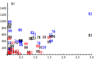
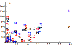
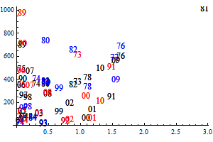
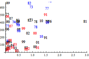
The historic performance of the default assessment is shown in figure 8
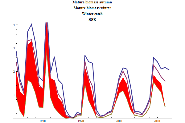
Figure 8. Historic performance of the Bifrost default assessment.
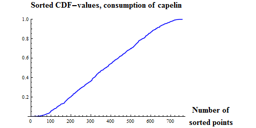 |
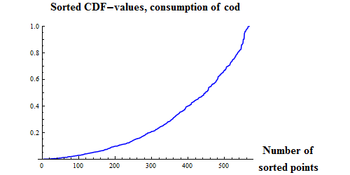 |
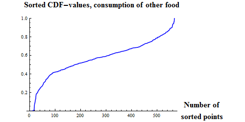 |
Figure 9. Q-Q plots for the consumption of capelin (upper), cod (middle) and other food (lower) by cod.
Recruitment functions
Introduction to recruitment
The long term simulations needed to test harvest rules are critically dependent on the relation between spawning stock and recruits that is used. Harvest rules aiming for MSY hinge around the marginal value of the spawning stock: if we catch an extra tonne, would the long-term detrimental effect through reduced recruitment outweigh the value o the extra catch? A glance at plots over recruitment vs. SSB for many fish stocks does not give much hope for evaluating the value of the spawning stock for future reruitment. However, the erratic influence from the environmen may effectively mask a possible spawning stock-recruitment relationship. The great importance of revealing the value of the spawning stock justifies much work being put into the study of recruitment relations. One might ask: if the SSB in a particular year had been higher, would the resulting recruitment also have been higher?
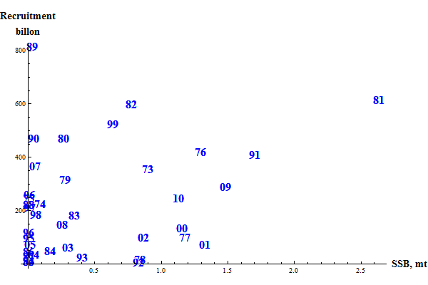
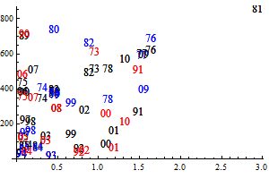
Figure 10. SSB-recruitment plot for the default Bifrost assessment.
The figure gives a general impression of larger recruitment at larger SSB. However, there are instances of large recruitments at very low values of SSB and of small recruitment at intermediate values of SSB. Small changes of the values might lead to rather large changes in the parameters estimated for e.g. a Beverton-Holt recruitment function. Taking the points at face value, theBeverton-Holt halfvalue is estimated at 0.013. Ommitting points with SSB < 0.08 (with the 1989 oint still in) the halfvalue is estimated at 0.154 and ommitting points withh SSB < 0.10 it is estimated at 1.48. A correct estimation of SSB at small values is thus of paramount importance for the results of long-term simulations.
The spread of the recruitment points can partly be explained by other covariates than SSB. In order to minimize model error as much as possible, a large number of recruitment functions are estimated and compared using the small-sample Aikaike Information Criterion (AIC, Burnham and Anderson 1998, p 66). In selecting recruitment forms and covariates the following considerations have been made:
Non-SSB covariates
We do not a priori know which other factors than SSB that affect the rescruitment in a particular year. The idea followed here is to test a suite of covariates and see which one(s) that have the best explanatory power using (small sample) AIC. The covariates below are tried:
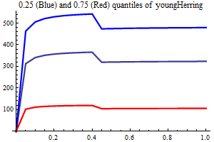
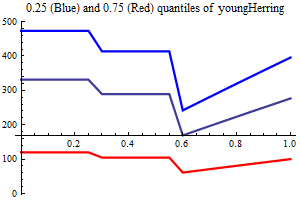
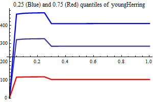
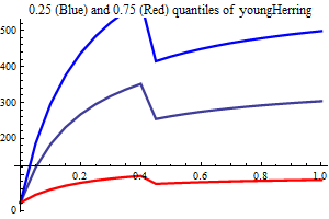
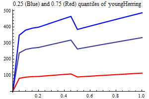
Young herring abundance
History suggests strongly that large yearclasses of Norwegian spring spawning herring may have a very strong influence on capelin recruitment. The herring abundance is taken from a herring assessment made with the model SeaStar rigged as closely as possible to the model TASACS used at present with management of the herring, since herring surveys in the Barents Sea exist have proven to be quite unreliable. The abundance in numbers have been converted to a scalar index by multiplying each age group with a fixe weight. Only ages 2 and 3 are used, and each herring of age 3 counts twice as much as each herring of age 1.
It is assumed that only herring abundances above a threshold influence capelin recruitment, and several threshold are tried, including 0. When herring abundance is a covariate and the threshold is larger than zero the estimation is performed in two steps, the first step estimating non-herring parameters, the second estimationg herring parameters keepingnon-herring parameters fixed at their estimated values. If the number of parameters is larger than 75% of the nunber of data points in either step the estimation is rejected.
As a separate covariate also zerogroup herring abundance is used.
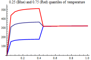
Environment
Temperature
AO index
Non-SSB covariates in the Beverton-Holt half value
The idea of using other covariates than SSB is that e.g. temperature may affect recruitment and including it in the recruitment relation may help reduce the uncertainty and get a clearer picture of the marginal value of the spawning stock. Usually, the effect of covariates are included multiplicatively i.e. the effect is the same for all values of SSB. There may be biological reasons for the effect to be larger at small values of SSB, which to some extent could be realized by letting the covariate be additive to the Beverton-Holt halfvalue. If the SSB always has a marginal value, i.e. if SSB in a particular year was larger the recruitment also would have been larger, covariates in the halfvalue could be a powerful way to model recruitment. Years in which the (yearly) additions to the halfvalue were small would be percieved as years with high recruitment success and large additive values would correspond to years with low recruitment success.
A word of caution
Some covariates giving a good fit may be spurious. For instance, including temperature as covariate will always improve the fit. However, there may have been systematic changes in geographical distribution over the same period as the temperature has changed systematically and the increased fit may have occured because the temperature then is a proxy for e.g. changed predation.
Variants of model form and uncertainty
Modelling median instead of expectation
It is difficult for the realized model to meet the assumed distribution - the nature defies normally our attempts to harness the recruitment process by our models. The ordinary approach is for the model to represent the expectation value in some distribution (most often log-normal). If it is more important to model the median right - as would be the case if a fishery in many years is more important than a high avarage long-term catch - an alternative approach could be to let the modelled for represent the median and not the mean. This is an option in the Bifrost suite of recruitment models.
Model form split at a certain value of SSB
Constant expectation of recruitment below an estimated SSB-limit
Positive intercept with the y-axis
In addition to the traditional Beverton-Holt formulation where recruitment goes to zero as SSB goes to zero, using an intercept with the y-axis is investigated. This is unbiological, of course, since an SSB at exactly zero will give a recruitment of zero. The interpretation is that we give up decsribing the recruitment relation very close to SSB = 0, and the intercept is an expression for the mean recruitment at small values of SSB, the part of the recruitment that does not depend on SSB.
Different uncertainty below and above a certain value of SSB
Environmental influence only below a certain value of SSB
Environmental influence on recruitment may be more important for capelin for spawning biomass levels below some value, as might be the case for cod (Brander 2005). For this reason, several threshold values has been tried, including a large enough value for environmental influence to occur over all ranges of SSB. It should be considered to include this as a parameter to be estimated - if many enough are tried it may be some cheating of the Akaike criterion. The threshold value can also be a vector of 2 elements, in which case the environmental effect is tapered off to zero between the two values.
Only influence of temperature below or above the median
Summary of estimation of recruitment functions
| Number of models | 13432 | 6172 | 14720 | 6247 | 6198 | 6087 | 6022 | ||||||||||||||
| medianTag | |||||||||||||||||||||
| uncertaintyTag | |||||||||||||||||||||
| dualModelTag | Dumod20 | ||||||||||||||||||||
| interceptTag | Intercept | Intercept | |||||||||||||||||||
| rangeTag | Upper | Upper | Upper | Upper | |||||||||||||||||
| constantBelowTag | ConstBel | ConstBel | |||||||||||||||||||
| File date Year,Month,Day |
{2013, 5, 10} | {2013, 4, 27} | {2013, 5, 9} | {2013, 4, 20} | {2013, 4, 27} | {2013, 4, 21} | {2013, 4, 21} | ||||||||||||||
| Smallest AIC | 68.756 | 73.597 | 73.67 | 72.739 | 73.946 | 74.282 | 73.704 | ||||||||||||||
| Half recruitment | .0080000000000000002` | 49.953 | .26700000000000002` | 21.961 | 0. | .20899999999999999` | {0.00900802, 19.1015} | ||||||||||||||
| Intercept | 0. | 0. | 0. | 0. | .97299999999999998` | 21.371 | 0. | ||||||||||||||
| SSB limit for constant below | 0. | .57300000000000006` | 0. | .66800000000000004` | 0. | 0. | 0. | ||||||||||||||
| Constant recruitment below | 0. | .049000000000000002` | 0. | .045999999999999999` | 0. | 0. | 0. | ||||||||||||||
| Rsquared | .74199999999999999` | .753` | .61299999999999999` | .75900000000000001` | .72399999999999998` | .72099999999999997` | .752` | ||||||||||||||
| Log-likelihood | -28.268 | -27.559 | -29.22 | -27.13 | -29.358 | -29.526 | -27.613 | ||||||||||||||
| Herring included | True | True | True | True | True | True | True | ||||||||||||||
| Temperature included | True | True | True | True | True | True | True | ||||||||||||||
| AO included | False | False | False | False | False | False | False | ||||||||||||||
| lowHerringAbundanceLimit | 0. | 0. | .40000000000000002` | 0. | 0. | 0. | 0. | ||||||||||||||
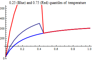
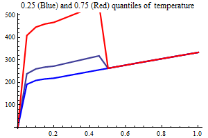
| Largest SSB env. influence |
.40000000000000002` | .25` | .25` | .40000000000000002` | .25` | .40000000000000002` | .25` | ||||||||||||||
| Factors in halfvalue | {} | {} | {} | {} | {} | {} | {} | ||||||||||||||
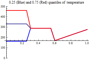
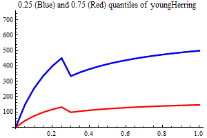
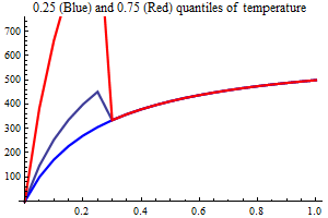
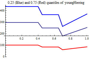
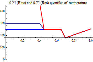
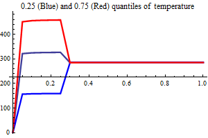
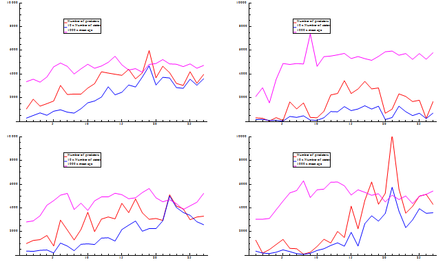
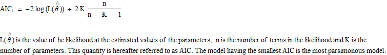
| Recruitment plots |
|
|
|
|
|
|
|
||||||||||||||
| SSB influence plots |
|
|
|
|
|
|
|
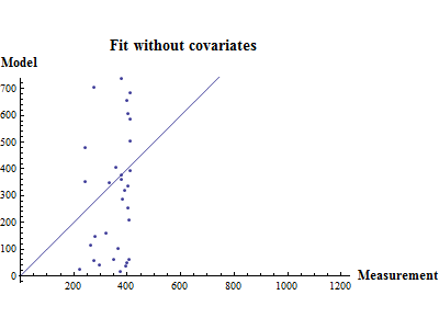
Figure 10. shows the fit between the best model (lowest AIC) and the data together with the fit obtained using a recruitment model without any other covariates than SSB.
 |
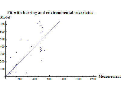 |
Figure 10. Model vs. data fit for a recruitment model without any other covariates than SSB (upper) and model vs. data fit for the best recruitment model, where herring and environmental indices are covariates.
Growth and maturation in prognostic runs
Estimation of parameter in growth and maturation models
The parameters governing growth and maturation are estimated prior to prognostic runs using a separate button on the menu. The models are linear and a standard method for linear estimation is performed. Parameters having a p-value of larger than 0.1 in the parameter table t-test are removed and the estimation is performed anew. All estimations with statistics and response plots are put to a separate notebook. Estimating anew to study the details on this notebook does no harm.
Stabilizing growth and maturation
10% and 90% quantiles in historic growth and maturation
Testing of harvest rules
Harvest rules are in Bifrost tested by long term simulation (several hundred years) over several historic replicates and several prognostic replicates. The mean long term yield and other management-relevant quantities are recorded for different values of HCR parameters.
Settings for long term simulations
Minimum SSB
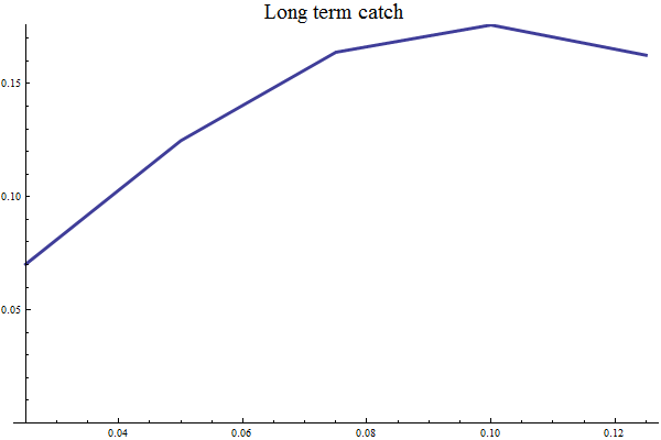
Figure 11 Mean long term catch as function of target SSB
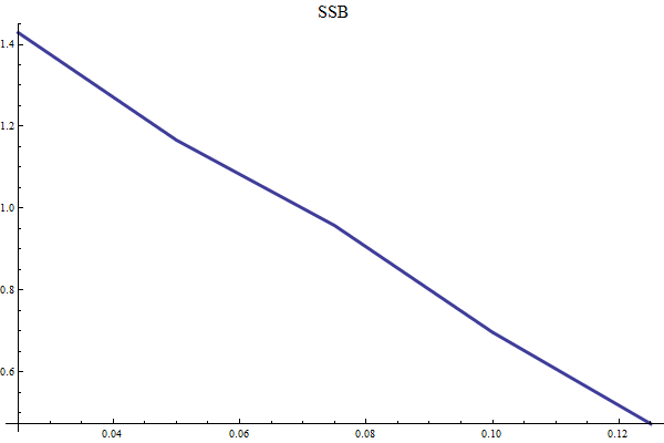
Figure 12 Mean long term SSB as function of target SSB
Maintenenace and development
Step-wiise instructions for updating
Estimation of parameters
| Step | How to |
| Verify that the estimation has converged | Use the parameter sequence table written on the project notebook during estimation |
Tricks of the trade
| Investgate | How to |
| Likelihood components as function of parameters | Button on main menu |
A note on the future
The revised model was run at the 2012 assessment meeting in Svanhovd and the HCR yielded a catch quota of 140 000 tonnes. The existing CapTool model yielded a catch quota of 200 000 tonnes. However, the change in methodology is substantial and the revised model has not been through an ICES benchmark process, so a TAC of 140 000 tonnes can hardly be put forward as ICES advice. The difference in the two quota suggestions points to an urgent need for a benchmark on the new methodology. In a bencmark process the biological and statistical ground for the revised method could be covered more widely than has been done in the present WD.
The Icelandic capelin is due for a benchmark revision as well, and these two stocks might be covered at one meeting.
The Norwegian-Russian fisheries commission has decided to revise Barents Sea HCRs by 2015 and by then the methodology should be extended to also include estimation of recruitment functions and testing of different HCRs including the MSY approach, possibly also with cod as prey species. This would make it possible to test joint cod-capelin HCRs.
In connection with renewal of capelin modelling personnell at IMR, a process of building new software based on AD Model Builder and R has started, which will give the technical basis for the methodology a more "standard" foundation.
Documentation
The most iportant documentation is of course the source code. In addition, teher are two primary sources of documentation, the present documentation note and documentation of part of the process available from the menu. Here, explanations of routines parametersand settings cam be listed and dispalyed graphicall, and textual documentation and plots for various parts of the process from implementation of data to evaluation of harvest rules is presented.
References
Brander, K.M. 2005. Cod recruitment is strongly affected by climate when stock biomass is low. ICES Journal of Marine Science, 62: 339-343.
Burnham, K.P. and D.R. Anderson. 1998. Model selection and inference: a practical information-theoretical approach. Springer-Verlag, New York, Inc. ISBN 0-387-95364-7
Jobling. M. 1988. Model selection and inference: a practical information-theoretical approach. Aquaculture, 70, 1-19.